Result Analysis Signal Modes (Added in Version 22)

A description of the theory of the calculation of the Transient Result Analyzer Modal Calculation is in a separate topic.

When performing results analysis on defined Transient Stability Result Analaysis Time Windows, with every signal being analyzed and PowerWorld will determine a trending line and a contribution of every mode to each signal, with the contribution described by a complex number. These values are summarized for all signals on the Result Analyzer - Damping\Signal Dmaping and Modes portion of the Transient Stability Dialog.

When looking at all the signals, the display is filtered to show only the contingency chosen from the contingency drop-down shown in the red box below. In addition to make filtering by particular time windows easier, there is a display listing all time windows in the blue box below. By checking or unchecking particular time windows the list of signals is filtered. Each row in the table represents a particular field of a particular object and we call each of these rows a "TSResultAnalysisSignal". As you click on a row in the table of signals, a second case information display to the bottom left is updated to show you information about all the Modes and their contribution to the signal you're looking at. In addition if you Auto checkbox is checked just above the list of modes on this dialog then as you click on rows in the upper table the bottom right portion of the dialog will update a display showing you the raw data of the signal in blue (the actual results from transient stability) and the approximate reproduced signal in red.

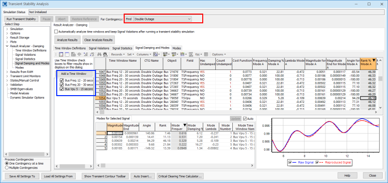
There are many fields which can be added to the case information display of signals. As with all case information displays you may configure the display to show many more columns than are added by default to the display. See the Configuring Case Information Displays for more information about how to add those. Of special not with this display however are the following columns

Time Window Name

Name of the Time Window for which the signal was calculated.

CTG Name

Name of the Transient Contingency from which the transient results were obtained

Field

The field for the signal

Object

The object for the signal

Trend Line For Signal

There are 3 fields to show the A, B, C coefficients of the trend quadratic function.

Cost Function Value

This is a measure of how closely the approximated signal matches the actual signal. Sort by this to see which signals match the worse. If the plot in the bottom right looks reasonable accurate then you know that even the worse match is pretty good. If the plot in the bottom right looks bad, then you may need to change the Time Window definition to change the time window to not include discrete jumps or increase the maximum sample frequency to improve the match.

Undamped Modes Has

Value will show a YES if the undamped mode count is greater than 0

Undamped Modes Count

A count of the number of modes within the signal that meets the UndampMinHz, UndampDampPerc, and UndampMinRank as defined by the Time Window

Modes by Sorted Magnitude

Provides information about the ModeMagAngle objects sorted by magnitude. Shows the Angle, Damping Ratio Percentage, Frequency, Lambda, Magnitude End, Magnitude, Mode Index, and Rank Percentage for every mode's contribution to this signal. The values are referred to as A, B, C, etc to represent the sort order.

Modes by Mode Index

Object Fields

There are various fields to show information about buses, areas, zones, and so forth for the object related to the signal.

Statistics

This folder contains the statistics which appear as default columns on the Signal Statistics tab.

If you right-click on a particular Signal and choose Show Dialog you will see information about only one signal. This shows information about the Time Window at the top of the dialog as well as the Contingency, Object, and Field related to the Signal. After this is a list of contributions of each mode to the signal being shown. The contributions are called TSResultAnalysisModeMagAngle objects. The first columns shown is Mode Include Reproduced and as you toggle those fields between YES to NO it impacts which mode contributions are included in the reproduced signal visualized on the right. When including all the contributions the reproduced signal should reasonably match the Raw signal if the Modal Analysis has worked well.

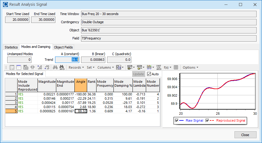
The columns shown with the contributions from each mode are as follows.

IncludeReproduced

Set to YES to Include this mode when calculating the reproduced signal from the modes and showing that in the user interface.

Magnitude (Mag)

Magnitude at Start Time for mode within Signal

Magnitude End (MagEnd)

Magnitude at End Time for mode within Signal

Angle

Angle for mode within Signal in degrees

Rank

This is the rank contribution of this mode to this signal based on the magnitude. It's based on the large of either Mag or MagEnd and is then normalized across all modes for this particular signal such that the summation of Rank values is 100.

Mode Frequency (Freq)

For Mode: Frequency of the mode in Hz

Mode Damping % (Damp)

The damping ratio percentage. This is 100 times the damping ratio which is equal to -100*Lambda/sqrt(sqr(Lambda) + sqr(2*pi*Frequency))

Mode Lambda (Lambda)

Exponential term for the mode which represents the damping. Negative Lambda indicates positive damping

Mode Number (Number)

Number of the mode. Number as just assigned by the calculation tool in no particular order

To demonstrate how toggling the IncludeReproduced field results in the reproduction of the raw signal see the following example.

Notice in the example that the 0.000 Hz mode in Row 4 is undamped because it has a positive lambda and thus negative damping percentage. However, this mode is not really representing an oscillation but is instead just slightly bending the curve to match the signal of the time window chosen. This would be ignored when considering whether the overall signal is damped or not.

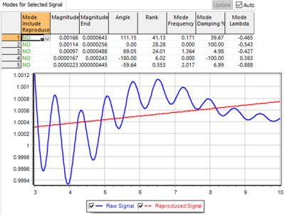
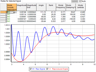
Toggle all the IncludeReproduced to NO in this example shows only the trend line of the signal.	Now add in the 0.171 Hz signal from Row 1 which gives the general shape of the signal only.

Now add in the 0.000 Hz signal in Row 2 which improves the match of the signal at the beginning of the signal	Now add in the 0.000 Hz signal in Row 4 which improves the match of the signal at the end of the signal.

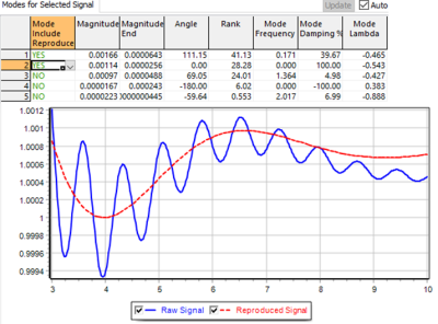
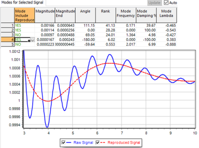
Finally add in the mode from Row 3 which includes the higher frequency 1.364 Hz oscillation. All these added together have reproduced our signal almost exactly.
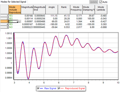