PV Curves Setup: Advanced Options

 

These options are found on the Advanced Options sub-tab located on the Setup tab of the PV Curves dialog. These options only apply when using Injection Group Ramping.

 

 

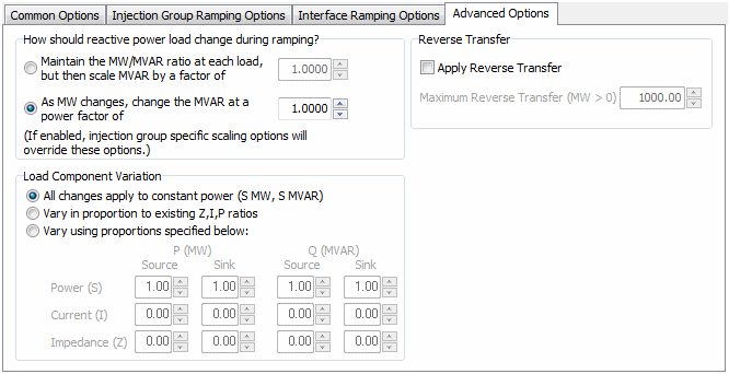
The power transfer that occurs during the PV analysis is a real power (MW) transfer. Loads can be specified as part of either the source or sink injection group that define the transfer. When loads are included in the transfer, the default is to only adjust the real power (MW) component of the load and leave the reactive power (Mvar) component constant. If any change is made to the reactive power load (Mvar) during the transfer, the default is to have all changes be made to the constant power component of the load. The Advanced Options tab allows specification of load variation for both real and reactive load to be something other than the defaults during the transfer.

The transfer amount and how the transfer is adjusted are determined by options found on the Common Options tab.

 

How should reactive power load change as real power load is ramped?

Total read power load changes, ΔP, at each load are determined based on the load's participation factor as defined with its associated injection group and the amount of transfer that is being implemented. ΔP is then used in conjunction with the selected reactive power change option to determine the associated total reactive power change, ΔQ, at each load.

Maintain the MW/MVAR ratio at each load, but then scale MVAR by a factor of

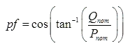
The total reactive power change, ΔQ, is determined based on the power factor, pf, at each nominal load (P_nom,Q_nom) prior to the load change and the change in total real power load, ΔP, due to the transfer. The power factor is determined by the following:

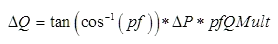
An additional multiplier, pfQMult, can be specified in order to modify the total reactive power load change to allow adjustment away from the present power factor. This multiplier is 1.0 by default. The change in reactive power load is then:

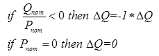
Maintaining a constant MW/MVAR ratio implies a sign convention that is lost when applying the arctan function to the ratio. An additional check is done to make sure that the calculated ΔQ is in the correct direction (maintains the correct leading or lagging power factor).

When loads are specified as constant power, constant current, and constant impedance components (ZIP components) rather than simply all constant power, the total load becomes a function of voltage. Maintaining a constant power factor at each load requires that we use nominal load (load at 1.0 pu voltage) that does not change as a function of voltage. When only constant power components are specified, the actual load is the same as the nominal load. Therefore, in all situations the power factor is determined based on the nominal load.

As MW changes, change the MVAR at a power factor of

This option allows the specification of power factor, pf_specified, for defining the total reactive power change, ΔQ, at a load. The change in reactive power load is then dependent on the change in total real power load due to the transfer, ΔP, and this specified power factor.

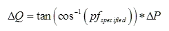
For this option, ΔQ is assumed to be in the same direction (has the same sign) as ΔP .

Injection groups have their own set of options that can override the options on this dialog if they are in use. See the Injection Group Specific Scaling Options topic for more information.

 

Load Component Variation

The total real power load change, ΔP, at a load during a PV transfer is determined by the load's participation factor as defined with its associated injection group and the amount of transfer that is being implemented. The total reactive power load change, ΔQ, is determined by the option selected for how reactive power should change during ramping as explained in the previous section. Total load change, (ΔP,ΔQ), at a load can be broken into ZIP components for constant power (ΔP_S,ΔQ_S), constant current (ΔP_I,ΔQ_I), and constant impedance (ΔP_Z,ΔQ_Z). During the PV transfer, the user can specify how changes in load due to the transfer should be split among these components.

The constant current and constant impedance components are a function of voltage and the nominal values specified for these components. Because of this, it becomes important to determine the load changes for the components based on nominal voltage and then apply these changes to the nominal components.

All changes apply to constant power (S MW, S MVAR)

All changes to load will be made to the constant power component:

The constant power component of load is not dependent on voltage so the total load change can be applied directly to the constant power component.

Vary in proportion to existing Z,I,P ratios

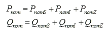
This option will change the load at a given load such that the ratios of the ZIP components do not change during the load adjustment. The existing ZIP ratios at a load are determined based on the present nominal load prior to any change due to the transfer. The existing total nominal power (P_nom,Q_nom) at a load is the sum of the components:

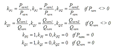
The component ratios are simply the ratio of each nominal component to the total nominal load at a load:

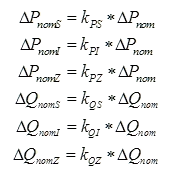
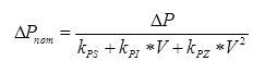
The resulting change in nominal load for each load component at a load is then the product of the ratio of each component and the total nominal power change:

Where the total nominal power change is determined from the total power change required at a load as a function of the present voltage, V, at the bus:

ΔQ_nom is calculated from ΔP_nom based on the selection of the option on how reactive power should change during the ramping as described in the previous section.

Vary using proportions specified below:

The factors are divided into four groups: real power load in the source injection group, real power load in the sink injection group, reactive power load in the source injection group, and reactive power load in the sink injection group. Each of these groups determines how the various components will change based on whether the load change is being done to real or reactive load and whether the load is part of the source or sink injection group. The default setting for each group is to apply changes only to the constant power component; Power (S) factor is 1 while all other factors are 0. The sum of the factors for each grouping must add up to 1. The Impedance (Z) factors are not enterable and are calculated to ensure that the sum is always 1. Simply adjust the Power (S) and Current (I) factors to appropriate values and the Impedance (Z) factor will be set automatically.

The calculation for determining the change in load components is done the same as described above when using existing ZIP ratios except that the ratios are user-specified here.

 

Reverse Transfer

The standard way of performing a PV analysis is to increase a transfer from the source to the sink in positive step increments determined by the Initial Step Size and other parameters that control the size of the step. When a contingency does not solve at zero transfer (base case conditions), it might be possible to find a solvable point by adjusting generation and/or load in the system. The Reverse Transfer option will attempt to find this solvable point by increasing a transfer from the sink to the source (instead of source to sink). This is done by incrementing the transfer from the source to the sink in negative step increments, effectively making the transfer go from the sink to the source.

When the Apply Reverse Transfer box is checked, an attempt will be made at finding a solvable point by applying the reverse transfer (sink to source) for any contingency that will not solve at zero transfer. A condition for this option to be used is that the base case power flow must solve.

When choosing to attempt the reverse transfer for contingencies that will not solve, all unsolvable contingencies will be processed even if the number of unsolvable contingencies exceeds the number of critical scenarios specified on the Results tab. The reverse transfer process will be done for all unsolvable contingencies prior to the standard PV process. After the reverse transfer process completes, the standard PV process (positive transfer from source to sink) will be performed on all contingencies that do solve at zero transfer level as long as the number of critical scenarios specified is not exceeded already by the number of contingencies that wouldn't solve as zero transfer.

The initial step magnitude by which the transfer is increased is the Initial Step Size specified with the Common Options. When a transfer level is found at which a contingency will solve, the step magnitude is reduced by the reduction factor specified with the Common Options. This is done in an attempt to find the minimum transfer required to reach a solvable point. This process will continue until a solvable point is found for each contingency of the Maximum Reverse Transfer (MW > 0) threshold is exceeded. It is likely that no solvable point can be found for some contingencies. The Maximum Reverse Transfer threshold should be set such that a reasonable transfer amount is attempted before abandoning the attempt at finding a solvable point. This process could be very time consuming if there are a number of contingencies that do not solve at zero transfer.

In addition to attempting to find a solvable point, the reverse transfer process can also attempt to find a solvable point at which all voltages are considered adequate. To check for adequate voltages during the reverse transfer process, check the option to Stop when voltage becomes inadequate that is found on the Limit Violations tab of the PV Curves dialog. This will force the process to find a reverse transfer point at which the contingency solves and all voltages are above the voltage level specified as inadequate. The inadequate voltage level is specified with the Voltage level to consider inadequate option also found on the Limit Violations tab.

If a reverse transfer point is found at which a contingency will solve, and voltages are adequate if choosing to include that check, the results for the scenario will list the Critical Reason as SRT - original critical reason with original critical reason being the reason why the contingency was considered not to be solved at the zero transfer level. The Max Export, Max Import, and Max Shift values that are reported are the minimum (in magnitude) transfer levels at which the contingency will solve and any voltage conditions are met. Values for any parameters that are being tracked through Quantities to Track will also be recorded at this transfer level. If there are multiple steps at which the contingency will solve and any voltage conditions are met while trying to find the minimum step, multiple transfer level points will be recorded making it possible to plot a few points of a PV curve.

If during the reverse transfer process no point can be found for which a contingency will solve and voltage conditions are met, the original results will be reported as if the reverse transfer process was not attempted.

If enforcing generator MW limits and/or not allowing negative loads during the transfer causes either the source or sink to not have enough resources to meet the required transfer, two other Critical Reason messages are possible. If the sink is maxed during the transfer, the Critical Reason will be given as RT Sink Maxed - original critical reason. If the source is maxed during the transfer, the Critical Reason will be given as RT Source Maxed - original critical reason. The Max Export, Max Import, and Max Shift values reported will be the values at which either the source or sink hit limits. Either of these messages indicates that the contingency will not solve or voltage conditions are not met, but the reverse transfer cannot continue because there are not enough resources in either the source or sink to do so. If either the source or sink is at its limits the contingency solution will still be attempted. If the contingency does solve and the voltage conditions are met, the Critical Reason will be given as SRT - original critical reason.

When the reverse transfer process completes, the system state is returned to the base case state in place when the PV analysis was first initiated. No reverse transfer amount will remain in the system state upon completion of the reverse transfer process even if the analysis is such that only the reverse transfer process is completed and no forward transfer scenarios are attempted.