OPF Reserves Example
In this section, we present an example of the OPF Reserves in action. Consider the 10 bus, 7 generator case contained in the B10Reserve.pwb case (included with PowerWorld Simulator). This case has 2 areas and 3 zones.
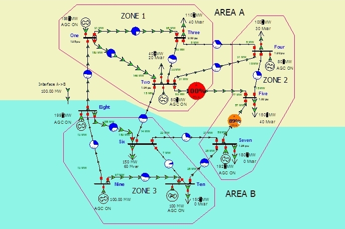
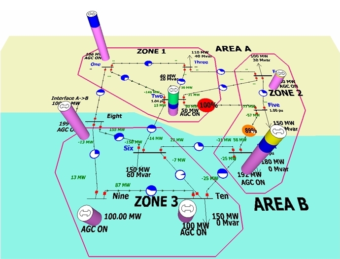
First solve the LP OPF without reserves by clicking LP Primal from the Add Ons ribbon group. Check the log to confirm a successful OPF solution. The initial LP OPF solution without reserves presents a binding transmission line as shown in the Figure.
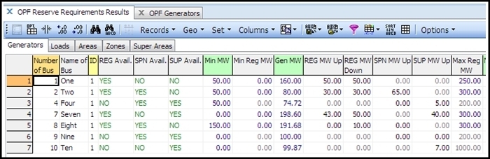
The first step to solving the OPF with reserves is to set up the reserve control availability and reserve bids from the Add Ons ribbon group > OPF Case Info > OPF Reserves > Generators case information display. The following parameters, which in this example will be set up in a tabular manner, can also be set in the individual Generator Information dialog. Let us set regulation, spinning and supplemental generator reserve availability as follows:
| Gen | Reg. Avail | SPN Avail | SUP Avail |
|---|---|---|---|
| 1 | YES | NO | NO |
| 2 | YES | YES | NO |
| 4 | NO | YES | YES |
| 7 | YES | NO | YES |
| 8 | YES | YES | NO |
| 9 | NO | YES | YES |
| 10 | NO | NO | YES |
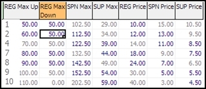
Then, let us set up the following reserve blocks and prices (reserve bids) in the same case information diagram.
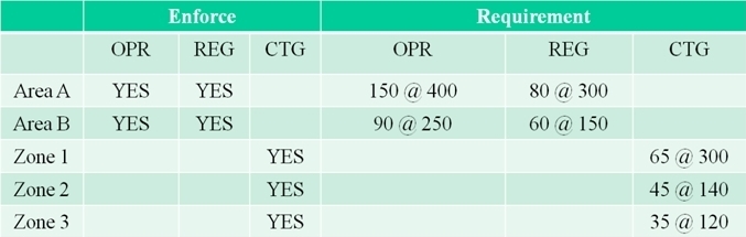
Once the generator and/or load reserve controls have been specified, the second step is to set up the reserve constraints for the control areas and/or zones. Let us set up the following data by accessing each individual Area Information dialog or Zone Information dialog. Recall, that a single level reserve requirement such as 150 MW @ 400 $/MWh is set by entering two points in the reserve demand curve: 0.0 MW at 400 $/MWh and 150 MW at 0.0 $/MWh.
Let us now solve the OPF enforcing reserve requirements. Go to the Add Ons ribbon tab and choose OPF Options and Results in the Optimal Power Flow ribbon group. Check the box Include OPF Reserve Requirements. Click the Solve LP OPF button from the dialog or the Primal LP button from the Add Ons ribbon tab.
The OPF Reserves, will enforce reserve constraints for each reserve type and for each area and zone whose Enforce Field is set to YES. In addition, OPF Reserve will observe the following constraints:
- Transmission line limits
- Generator MW Max and Min limits for the total energy plus reserve controls
- Area scheduled interchange. For this case, there is a 100 MW export from Area A to Area B.
To explore the results, go to the Generators page in OPF Reserve Results in the Model Explorer. The results include generator MW dispatch and assignment of all the reserve services. Note that in this example, some of the generators have reached their reserve bid limits for certain units and types of reserve.
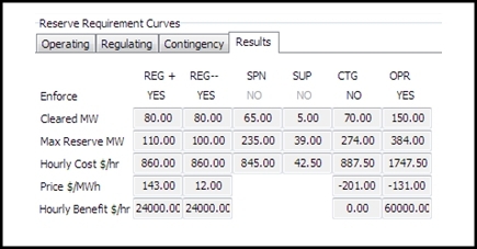
Results can be explored at the area or zone level by accessing the individual Area Information dialog or Zone Information dialog, going to the OPF tab, and the Results subtab of the Reserve Requirement Curves. For instance, the Results for Area A are as shown in the next Figure. For each area, the results page shows the enforcement of different types of regulation, the total cleared reserve, the total available reserve, the reserve cost per hour, the reserve price, and the hourly benefit, which corresponds to the area below the demand curve and above the equilibrium RMCP level.
The Results tab of the OPF Options and Results dialog shows the details of Bus MW marginal prices, including energy, congestion and losses, and the reserve prices associated with the area or zone reserve constraints. The corresponding linear programming details will list among the LP variables the reserve controls specified by the user. The LP tableau will include specific rows for the enforced reserve constraints at the area and zone level, etc. Reserve results can be visualized as any other generator, load or bus object field in Simulator.
It should be mentioned that OPF Reserves is fully incorporated with the Time Step Simulation (TSS) tool, so hourly OPF runs including reserves can be performed and results versus time stored. However, currently OPF Reserves cannot be used simultaneously with the SCOPF tool.