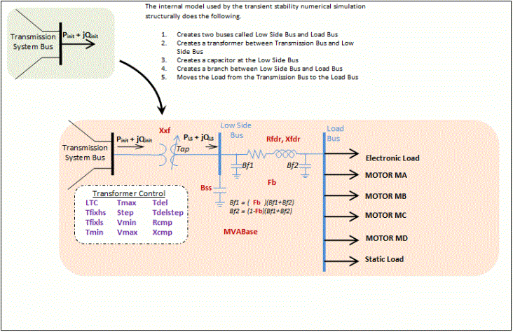
The create composite load model command allows you to transform the original transmission bus load wthat has a transient stability load model of CMPLDW into a distribution equivalent inside the power flow case. To append a case to the existing case, go to the Tools ribbon tab and choose Modify Case > Create Composite Load Model... from the Edit Mode ribbon group.
Below is a picture of how the original transmission bus load with a CMPLDW Transient Model is converted into a distribution equivalent inside the power flow case:

When creating the new element in the power flow and calculating the parameters of the distribution equivalent the following calculations are done
- The Low Side Bus will have a bus numer of 800,000 + the Original Transmission Bus number.
- The Load Side Bus will have a bus numer of 900,000 + the Original Transmission Bus number.
-
The created load records IDs to now be "MA", "MB", "MC", "MD" for the motors, "C1" for static load, and "PE" for the electronic load.
- A Distribution Equivalent MVA Base is determined based on the parameter MVABase.
- If (MVABase > 0) then DistEquivMVABase = MVABase
- If (MVABase < 0) then DistEquivMVABase = Pinit/MVABase
- If (MVABase = 0) then DistEquivMVABase = Pinit/0.8;
- The six impedance parameters (Bss, Rfdr, Xfdr, Xxf, Rcmp, Xcmp) of the Distribution Equivalent Type are assumed to be on this DistEquivMVABase and are converted the to the System MVA Base. For example, Xxf = Xxf * SystemMVABase/DistEquivMVABase.
- Transformer Taps and impedances are converted to the System MVA Base based on the fixed taps. (Note that the variable tab is assumed to be at the Low Side Bus).
- Xxf = Xxf * (Tfixhs)2
- Step = Step/Tfixhs
- Tmin = (Tmin + Tfixls - 1)/Tfixhs
- Tmax = (Tmax + Tfixls - 1)/Tfixhs
- The transformer tap ratio is assumed to be set such that the voltage at the Low Side Bus is equal to the average of Vmin and Vmax. The tap ratio is then rounded to the nearest discrete step and brought back within the Tmin - Tmax range if necessary.
- Using the impedances and taps now available, the Low Side Bus voltage is calculated exactly and the resulting flow on the Low Side Bus of the feeder is calculated exactly (PLS + jQLS).
- We now initially assume that Bf1 and Bf2 are both zero, and from this an estimate of the resulting flow reaching the Load Bus of the feeder is calculated as Pnew + jQnew and the resulting Load Bus Voltage as well.
- If the Load Bus voltage falls below 0.95 per unit, then the feeder impedances Rfdr and Xfdr are reduced by a factor that results in a Load Bus Voltage of 0.95 per unit. (Note: if the Low Side Bus Voltage is less than or equal to 0.95, then Rfdr and Xfdr are set to the minimum impedance values of 0.0000001 + j0.00001)
The perfectly initialized voltage at the Load Bus and the values of Pnew + jQnew cannot be immediately calculated. This is because they will depend on the initialization of the transient load model that is assigned to this load record. During the initialization of the load model the resulting extra Mvar values calculated due to motor initialization will be assigned to the feeder shunt values Bf1 and Bf2 according to the parameter Fb. In the simplest case when Fb = 0, all the extra Mvars are assigned at the Load Bus (Bf2) and thus the estimate of the voltage at the Load Bus will not change. When Fb > 0 however, this means that some of the Mvars are assign to the Low Side Bus (Bf1) and this will slightly impact the calculation of the Load Bus voltage and the values of Pnew + jQnew. To accommodate the splitting of this admittance the initialization routine must iteratively perform load initialization and the allocation of the split of Bf1 and Bf2 until it converges to a consistent solution. Throughout this iteration the restriction that the Load Bus voltage not fall below 0.95 per unit must also be maintained. This is all done internally by Simulator.