Load Characteristic Model: PERC1
Available in October 27, 2025 path of Version 24
PERC1 is an acronym for the Power Electronic Reconnecting and Ceasing load model. It is based on LDEV1 which was based on the model developed by EPRI summarized in the November 2022 report entitled
"A Positive Sequence Model for Aggregated Representation Electric Vehicle Chargers"
EPRI Project 1-116982
written by L. Sundaresh and P. Matra
This model is based on the LDEV1 model. PERC1 is appropriate to represent any aggregation of a large number of power electronic loads. Examples would be an electrical vehicle charging, a large number of computers such as a data center, a cryptocurrency mining facility, a large number of variable frequency drives, and so on. The differences between LDEV1 and this model are as follows
-
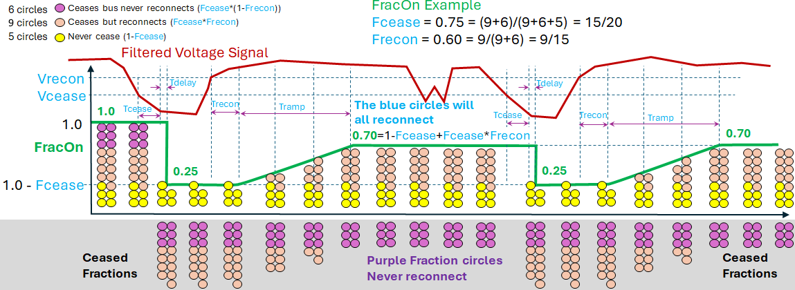
Frecon is provided so that after reconnecting is complete the fraction may not come back to 1.00 but instead to a reduced value of (1 - Fcease + Frecon*Fcease)
-
Tap, Tbp, Taq, Tbq: Separate Lead/Lag time constants are provided for the P and Q paths
-
Dbfl and Dbfh are separate parameters for low and high frequency deadband
-
Has a single path for P and Q instead of 4 fractional paths. Multiple PERC1 load models could be used with the CompLoad component-based load structure to model multiple paths.
Description of the PERC1 model
While the model developed by EPRI was for an electric vehicle charger model, this model can be used to represent any aggregation of a large number of power electronic loads. Examples would be an electrical vehicle charging station, a large number of computers such as a data center, a crypto-currency mining facility, a large number of variable frequency drives, and so on.
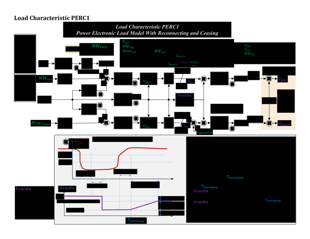
The values MWinit and Mvarinit on the left of the block diagram below are calculated as part of the stability simulation initialization routine. MWInit is set equal to the initial MW of the load. When this model is used inside the CompLoad component-based load structure, then the parameter QPRatio is used to calculate the Mvarinit value and any extra Mvars are assigned as done with the CompLoad. When this model is used as a stand-alone model as part of a LoadModelGroup, Load, Bus, Area, etc. then the QPRatio is ignored and the Mvarinit is set equal to the load's initial Mvar. If a simple event occurs in the simulation and the final voltage returns to the initial voltage and the cease and reconnect logic is never engaged during the simulation, then this model will bring the MW and Mvar back to the same as the initial condition. The top half of the block diagram below represents the real power (MW) response of the load while the bottom half of the block diagram represents the reactive power (Mvar) response.
The dynamic portion of this model is described in the left side of the block diagram by the dynamic states 1 - 6 . The washout blocks (Kvp/Tvp and Kvq/Tvq parameters) model a response where the model load will decrease when a decreasing voltage is encountered (such as after and during a fault) and the load will then increase when the voltage is increasing (during fault recovery). This is meant to model a device such as a variable frequency drive which may reduce the electrical power during a fault, but then after the fault clears an additional amount of load will be seen to re-accelerate the mechanical load that the VFD is driving. This model is not simulating any characteristics of the mechanical load or the control system that causes this behavior, but is using the simple washout blocks to approximation the behavior. The MW control path also includes a simple frequency droop with deadband response that the load may have. After this the lead lag blocks are used to model any other transient response of the real and reactive loads. This leads to States 1 and 2 in the block diagram below which represent the model's request for a per unit power based on the initial voltage Vinit.
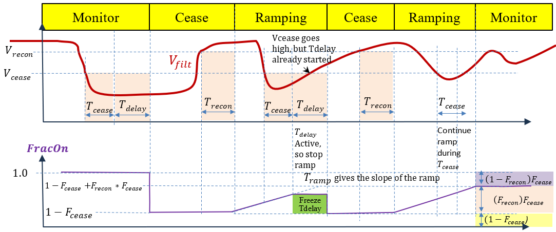
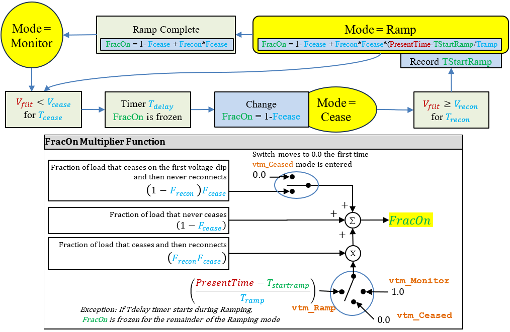
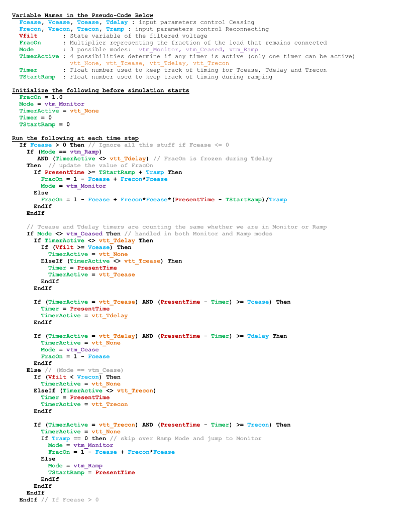
After this, both the real power and reactive portions of this model have a user input which is the exponent of the voltage relationship relative to the initial voltage. Any value of nP and nQ is allowed, but it is useful to realize that nP = 0 indicates a constant power at steady state, nP = 1 indicates constant current, and nP = 2 indicates constant impedance. After the exponent, it then divides by per unit voltage to convert to a current signal. The limits Ipmax/Ipmin or Iqmax/Iqmin are then used. Next the current is multiplied by a value FracOn which represents the fraction of the load that remains connected to the system. The FracOn models the Cease and Reconnect logic. If the filtered voltage is less than Vcease for more than Tcease seconds, then a decision to cease a portion of the load is made. Then, after an additional delay of Tdelay seconds, the FracOn is reduced to a value of (1 - Fcease). Then the system will wait to see if the filtered voltage goes above Vrecon for more than Trecon seconds at which time it will begin ramping the FracOn value back up over a time of Tramp seconds to a value of (1 - Fcease + Fcease*Frecon). Additional detail is included below to describe how these timers are reset and how a voltage drops after the model begins ramping is handled. See the pseudo-code and diagrams below for more details.
Finally, the output goes through another delay block using the Tt time constant to result a final desired current for each path. The treatment of this model in the algebraic network boundary equations is then a constant current.
Model Equations and/or Block Diagrams
Modified in Version 24 patch on February 11, 2026. Added the initialization feature Iqextra when the model is used as a stand-alone model.
| Parameter | Description | Default |
| Lfm | Loading factor used to calculate MVAbase of model as MWinit/Lfm. If Lfm < 0.001 then software will use a value of 0.80 |
0.80 |
| QPratio | Q/P ratio for MvarInit computation from MWInit. MvarInit = QPRatio*MWInit | 0.66 |
| Dbfl | Deadband on frequency response low (<=0) [pu] | 0.00 |
| Dbfh | Deadband on frequency response high (>=0) [pu] | 0.00 |
| Kdroop | Frequency droop [per unit] | 0.00 |
| Kvp | Proportional constant for active power washout | 0.00 |
| Tvp | Time constant for active power washout [seconds] | 0.10 |
| Kvq | Proportional constant for reactive power washout | 0.00 |
| Tvq | Time constant for reactive power washout [seconds] | 0.10 |
| Tap | Lead time constant for real power path [seconds] | 0.00 |
| Tbp | Lag time constant for real power path [seconds] | 0.00 |
| Taq | Lead time constant for reactive power path [seconds] | 0.00 |
| Tbq | Lag time constant for reactive power path [seconds] | 0.00 |
| nP | Active Power Exponential | 0.00 |
| nQ | Reactive Power Exponential | 1.00 |
| Ipmax | Maximum Ip [per unit] | 1.00 |
| Ipmin | Minimum Ip [per unit] | 0.00 |
| Iqmax | Maximum Iq [per unit] | 0.66 |
| Iqmin | Minimum Iq [per unit] | -0.66 |
| Fcease | Fraction that will cease (between 0 and 1) | 1.00 |
| Vcease | Voltage threshold for cease logic [per unit] | 0.50 |
| Tcease | Time delay for cease logic to be initiated for (>= 0) [seconds] | 0.01 |
| Tdelay | Time delay to cease after detection for (>= 0) [seconds] | 0.00 |
| Vrecon | Voltage threshold to initiate power ramp reconnection logic (Vrecon >= Vcease) [per unit] | 0.60 |
| Trecon | Time delay for ramp up logic to be initiated (>= 0) [seconds] | 0.05 |
| Tramp | Ramp up time (>= 0) [seconds] | 1.00 |
| Frecon | Of the Fraction that ceases, this is the fraction that then reconnects (between 0 and 1)t] | 1.00 |
| Tt | Time delay for outputs [seconds] (If < 4*TimeStep will be treated as 4*TimeStep) | 0.02 |
| Tv | Voltage measurement time constant [s] | 0.02 |
| Tf | Frequency measurement time constant [s] | 0.02 |